R project

Data

The data can be found by googling "open data atmosphere" and "meteocat open data":

Air pollution data & Meteorological data

From the meteorological data the codes of the variables that we need are 30 for wind speed that we will put ws, and 31 for wind direction that we will put wd. The dates will be in ISO8601 format 2021-03-15 16:00:00 with POSIXct format with the name date. The names date, ws and wd are Openair requirements.

Library

RStudio software and the Tidyverse and Openair packages must be installed.

Tidyverse allows you to sort the data. Openair allows hour by hour, day by day, year by year air studies in a specific and advanced way. To install these 2 R packages you must type:

install.packages (c("tidyverse","openair"))

Sort Data

We must read the data from our computer:

city<-read.csv ("C://Users/YOURCOMPUTERNAME/Documents/city.csv") 

View(city)

We change the times of the columns to rows using pivot_longer

city1<-pivot_longer(city,cols=c(h01,h02,h03,h04,h05,h06,h07,h08,h09,h10,h11,h12,h13,h14, h15,h16,h17,h18,h19,h20,h21,h22,h23,h24), names_to="hour", values_to = "value")

city2<-city1[-c(1,2,4,6:16)]

write.csv(city2,"C:\\Users\\YOURCOMPUTERNAME\\Documents\\city2.csv")

Modify data

We delete T00.00.00.000 and replace the times H01, etc for 01:00:00 until we get the dates in ISO format:

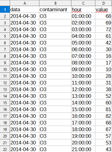
We associate date and time together to city4.csv using LibreOffice Calc or RStudio.

city4 <- city3 %>% mutate(name=paste0(data, " ", hour))

We create city5 by putting day and time together under the column name date

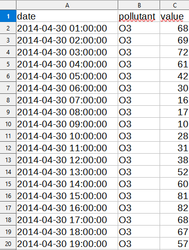
Convert data's format

library(openair)

city5PM10 <- subset(city5, pollutant=="PM10")

city5PM10$date<-as.POSIXct(city5PM10$date,"%Y-%m-%d %H:%M:%S", tz="Europe/Madrid")

class(city5PM10$date)

[1] "POSIXct" "POSIXt"

View(city5PM10)

class(city5PM10$date)

[1] "character"

city5PM10$date<-as.POSIXct(city5PM10$date,"%Y-%m-%d %H:%M:%S", tz="Europe/Madrid")

class(city5PM10$date)

[1] "POSIXct" "POSIXt"

class(city5PM10$pollutant)

[1] "character"

city5PM10$pollutant<-as.factor(city5PM10$pollutant)

class(city5PM10$pollutant)

[1] "factor"

Create graphics with Openair

timeVariation(city5PM10, pollutant="value")

trendLevel(city5PM10, pollutant = "value", main="PM10 evolution in MYCITYNAME")

daily<-timeAverage(city5NO2,avg.time = "day")
View(daily)
calendarPlot(city%NO2, pollutant="value", year="2020")

yearly<-timeAverage(city5no2,avg.time = "year")
View(yearly)

• Air quality standards indicate different pollution limit levels,for example, for NO2; levels must be below 40 µg/m3.
• We can check for example the number of exceedances of the eight-hour PM10 averages with this code:

library(openair)
episode<-selectRunning(city6, pollutant="PM10",threshold=40, run.len=12)
nrow(episode)

In this case, the answer is:

[1] 132

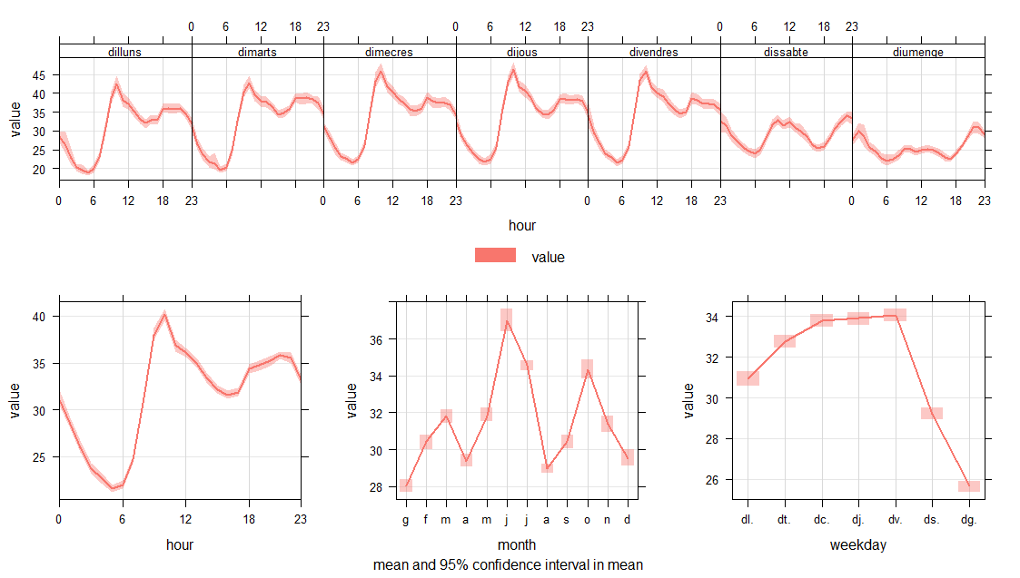
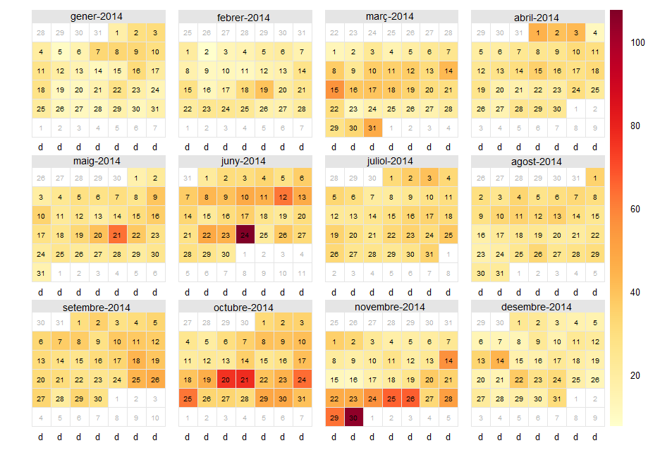
The program tells us that the level of 40 µg/m3 has been exceeded in the 12h average a total of 132 times.

Sort Data whit pivot_wider

library(tidyverse)
library (openair)
city6<-pivot_wider(city5, names_from= pollutant, values_from =value)
View (city6)
write.csv(city6,"C:\\Users\\YOURCOMPUTERNAME\\Documents\\MYCITY\\city6.csv")

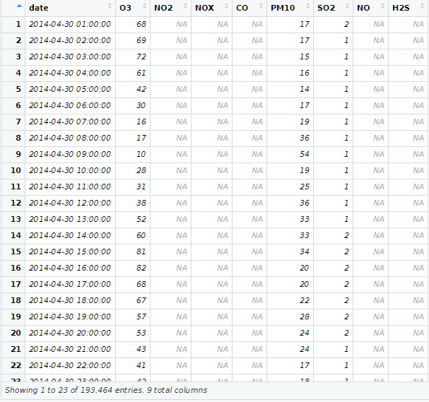
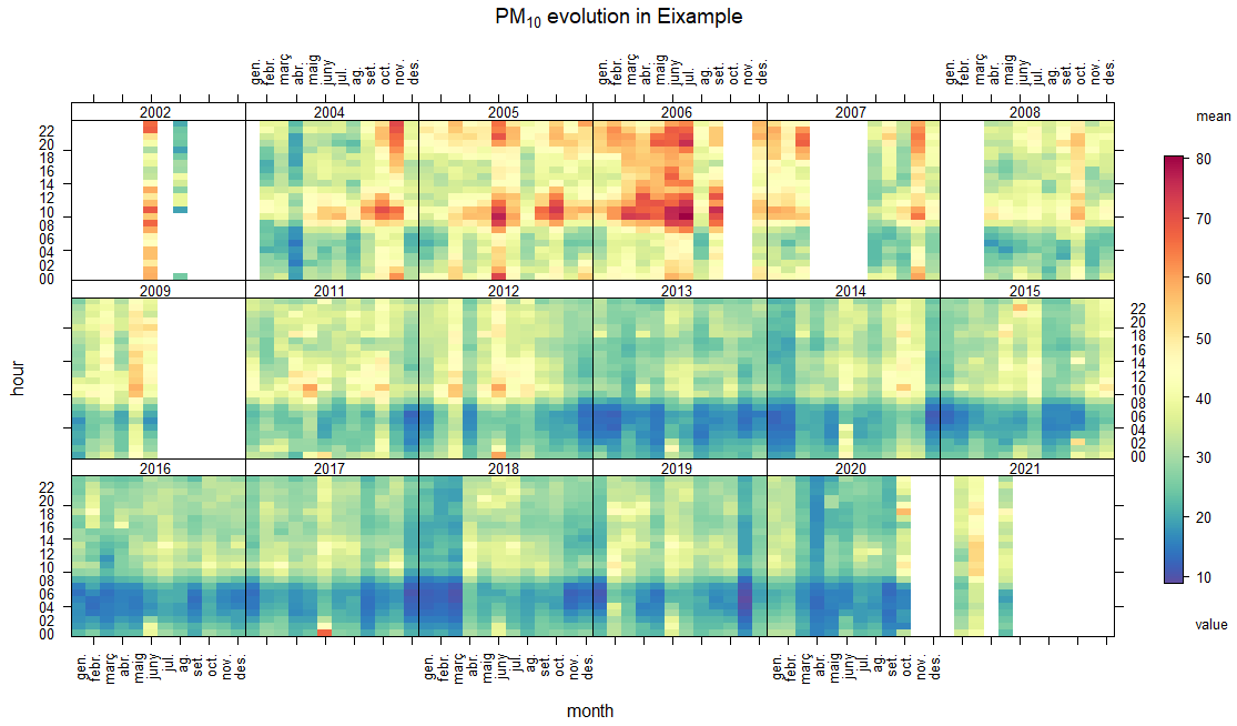
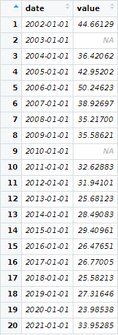
Time pollutant variation's 199X-20XX

class(city6$date)

[1] "character"

city6$date<- as.POSIXct(city6$date,format="%Y-%m-%d %H:%M:%S",tz="Europe/Madrid") 
timeVariation(city6, pollutant=c("NOX","NO2","CO","SO2","H2S","NO","PM10","O3", "HCT","HCNM"), main="Air pollution in MYCITY (1991-2021)")

Sort meteorological data's

wind<-read.csv("C://Users/YOURCOMPUTERNAME/Documents/wind.csv")

View(wind)

wind1<-wind[-c(1,2,5,7,8)]

wind2<-pivot_wider(wind1,names_from = CODI_VARIABLE, values_from = VALOR_LECTURA)

names(wind2)[names(wind2) == "31"] <- "wd"

names(wind2)[names(wind2) == "30"] <- "ws"

names(wind2)[names(wind2) == "DATA_LECTURA"] <- "date"

write.csv(wind2,"C:\\Users\\YOURCOMPUTERNAME\\Documents\\wind2.csv")

Linking the two data types

We have to be sure that the wind database date class is a POSIXct date type in order to combine it.

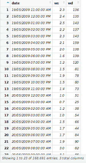
It can be joined using an Openair funcion:

 library (openair) 

 cityall<-merge(city6, wind6, by ="date") 

 View (cityall)

And now we can do pollutionRose and see where the pollution is coming from.